Josephus problem -- C versus J

In this post, we will see about implementation of a famous problem -- the Josephus Problem.

As you can see, there's already an implementation in mathematica. But, not many of us are rich enough to buy MM. So, we need to make use of awesome and free programming languages like C and J! C for fast execution, J for quick coding.

First, to implement in C, we need to write our own data structures. We will make use of a circular linked list, since that's how the josephus problem is stated.

#include <stdio.h>
#include <stdlib.h>

struct node *cur,*tmp,*head;
struct node
{
   int num;
   struct node *next;
};

void kill(int n, int k)
{
    struct node *prev;
    while(k>1){
        prev=head;
        head=head->next;
        k--;
    }
    tmp=head->next;
    free(head);
    prev->next=tmp;
    head=tmp;
}
int main()
{
    int n,k,i;

    scanf("%d",&n);
    scanf("%d",&k);
    head=(struct node*)malloc(sizeof(struct node));
    head->num=1;
    tmp=head;
    for(i=2;i<=n;i++)
    {
        cur=(struct node*)malloc(sizeof(struct node));
        cur->num=i;
        tmp->next=cur;
        tmp=cur;
    }
    cur->next=head;
    while(n>1){
        kill(n, k);
        n--;
    }
    printf("%d\n",head->num);
    return 0;
}

For the original Josephus problem, \(n=41\) and \(k=3\), and the program answers \(31\) as expected. Next, we move on to J:

J being an array programming language, there are verbs to operate on arrays. So, the josephus problem is a natural candidate for J. Here it goes:

1
2
3
a=:1+i.41
jose=: 4 : 'a=:}.(x-1)|.y'  NB. rotate and delete the first item
3 jose^:(_1+#a) a

There, very much smaller than the C version. J code above uses nesting of function, i.e. the function jose is applied 40 times on array 'a', and a single element remains after that.

A more explicit version can be written as:

1
2
3
4
5
6
7
    jos =: 4 : 0
while. (#y)>1 do.
y=.}.(x-1)|.y
end.
return. y
)
    3 jos 1+i.41

When n is small, the execution time does not make much difference either in J or C. But we can notice the difference clearly when n is large. E.g. for \(n=40000\) and \(k=11\), the time taken in J is about 1.68s and in C, it's only about 0.018s in my machine. J can be sped up a bit by operating on multiple items at a time, and makes the program a little more complicated.

You may wish to compare this with your favorite language's implementation in rosettacode, which has several clever solutions.

Applications of Generating Functions

Generating Function (g.f.) is one of the most important tools in combinatorics. Many problems which are difficult to do by combinatorial arguments and by cases are trivial when g.f. is applied. Below are some typical problems where g.f. are very useful.

1 Solving diophantine equations (d.e.)

  1. What are the number of solutions for the linear d.e.
\begin{align*} \displaystyle x_1+x_2+x_3+x_4=35\\ 1\le x_1,x_2\le 20\\ 20\le x_3,x_4 \le 30 \end{align*}

Answer can be easily found by representing the variables as polynomials and multiplying them, i.e.

\begin{equation*} \displaystyle [z^{35}](z+z^2+z^3+\cdots +z^{20})^2\, (z^{20}+z^{21}+z^{22}+\cdots +z^{30})^2 = 11 \end{equation*}

Hence, there are 11 solutions for the d.e under the constraints.

In Sage, this can be found by the taylor expansion:

taylor((x-x^21)/(1-x)*(x^20-x^31)/(1-x),x,0,35).coefficient(x,35)

We can even get a closed form if the problem is changed to

\begin{align*} \displaystyle x_1+x_2+x_3+x_4=n\\ 0\le x_1,x_2, x_3,x_4 \end{align*}

The g.f. for this is written as

\begin{equation*} \displaystyle (1+z+z^2+z^3+\cdots)^4=\dfrac{1}{(1-z)^4} \end{equation*}

and the nth coeffiecient is

\begin{equation*} \displaystyle [z^n]\dfrac{1}{(1-z)^4}=\dbinom{n+3}{3} \end{equation*}

b) Number of ways to make changes for n units using coins of denominations 1,2 and 5 units. The d.e. for this problem is written as

\begin{equation*} \displaystyle x_1+2\, x_2+5\, x_3=n \end{equation*}

and the g.f. is

\begin{equation*} \displaystyle G(z)=\dfrac{1}{(1-z)(1-z^2)(1-z^5)} \end{equation*}

The \(n^{th}\) coefficient gets the exact answer, but having a g.f. allows us to do more, like having an asymptotic form. In this case, factor the denominator

\begin{equation*} \displaystyle G(z)=\dfrac{1}{(1-z)^3}\cdot \dfrac{1}{(1+z)(1+z+z^2+z^3+z^4)} \end{equation*}

The first part of the two fractions contributes the most to the coefficients, and an approximation can be written as

\begin{equation*} \displaystyle [z^n]G(z)\sim [z^n]\dfrac{1}{(1-z)^3}\cdot \lim_{z\to 1}\dfrac{1}{(1+z)(1+z+z^2+z^3+z^4)} =\dfrac{\dbinom{n+2}{2}}{10} \end{equation*}

Comparing the precise and approximate answers: for \(n=1000\) \(50401\) and \(50150.1\),

for \(n=2000\) 200801 and 200301.1, respectively.

2 Partial and infinite sums

  1. Finding a closed form for
\begin{equation*} \displaystyle \sum_{k=1}^n k \end{equation*}

For problems like this, we can make use of the property of g.f:

\begin{align*} \displaystyle G(z)=\sum_{i\ge 0} a_i\, x^i\\ \implies \dfrac{1}{1-z}G(z)=\sum_{i\ge 0}\left(\sum_{j=0}^i a_j \right)z^i \end{align*}

G.f. for \(<0,1,2,3,\ldots>\) is given by

\begin{equation*} \displaystyle G(z)=\dfrac{z}{(1-z)^2} \end{equation*}

Hence, to find the sum, it's simply

\begin{align*} \displaystyle \dfrac{1}{1-z}\, G(z)=\dfrac{z}{(1-z)^3}\\ \implies [z^n]\dfrac{1}{1-z}\, G(z)=\sum_{k=1}^n k = \dbinom{n+1}{2} \end{align*}

We can then proceed to find more complicated sums like

\begin{equation*} \displaystyle \sum_{k=1}^n k^2 \end{equation*}

which are usually done in high school by mathematical induction, but never shown how to derive in the first place. To derive it from g.f., we must first find the g.f. for , which can be easily obtained by differentation. i.e.

\begin{equation*} \displaystyle z\, \dfrac{d}{dz}\left(\frac{z}{(1-z)^2}\right)=\dfrac{z+z^2}{(1-z)^3} \end{equation*}

and the sum of the squares is

\begin{equation*} \displaystyle [z^n]\dfrac{z+z^2}{(1-z)^4}=\dbinom{n+2}{3}+\dbinom{n+1}{3}=\dfrac{1}{6} \, {\left(2 \, n + 1\right)} {\left(n + 1\right)} n \end{equation*}

which can be verified by Sage

var('n');
show(factor(sum(x^2,x,0,n)))
  1. Summation of infinite series

For this purpose, the dummy variable in the g.f. is replaced by a constant to obtain the closed form. E.g. i)

\begin{equation*} \displaystyle \sum_{i\ge 0}\frac{1}{5^i} \end{equation*}

We have the g.f. for \(< 1,1,1,\ldots >\)

\begin{align*} \displaystyle G(z)=\dfrac{1}{1-z}\\ \implies G(1/5)=\dfrac{5}{4} \end{align*}
  1. We can also solve seemingly complicated sums like
\begin{equation*} \displaystyle \sum_{i\ge 0} \dfrac{i^2\, F_i}{12^i} \end{equation*}

where \(F_i\) is the \(i^{th}\) fibonacci term.

The g.f. for \(F_i\) can be shown to be (derived from the linear recurrence relation)

\begin{equation*} \displaystyle G(z)=\dfrac{z}{1-z-z^2} \end{equation*}

Next, obtain the g.f. for \(i^2 F_i\)

\begin{equation*} \displaystyle G_1(z)= z\, D\left(z\, D\left( \dfrac{z}{1-z-z^2} \right) \right) = \dfrac{z^5 - z^4 + 6\, z^3 + z^2 + z}{(1-z-z^2)^3} \end{equation*}

where \(D\) is the differential operator \(d/dz\) and

\begin{equation*} \displaystyle \sum_{i\ge 0} \dfrac{i^2\, F_i}{12^i} = G_1(1/12) = \dfrac{279804}{2248091} \approx 0.124462933217561 \end{equation*}

In Sage, it's written as

(x*diff(x*diff(x/(1-x-x^2),x),x)).subs(x=1/12)

3 As probability g.f. and obtain expected values

In probability g.f., the coefficients are the probability of occurance of the value. The p.g.f. for a die with 6 faces numbered 1 to 6 is given by

\begin{equation*} \displaystyle P(x)=\dfrac{x+x^2+x^3+x^4+x^5+x^6}{6} \end{equation*}

and the probability of the sums when two dice are thrown

\begin{equation*} \displaystyle P_2(x)=P(x)^2=\frac{1}{36} \, x^{12} + \frac{1}{18} \, x^{11} + \frac{1}{12} \, x^{10} + \frac{1}{9} \, x^{9} + \frac{5}{36} \, x^{8} + \frac{1}{6} \, x^{7} + \frac{5}{36} \, x^{6} + \frac{1}{9} \, x^{5} + \frac{1}{12} \, x^{4} + \frac{1}{18} \, x^{3} + \frac{1}{36} \, x^{2} \end{equation*}

and the expected value shown when the die is thrown:

\begin{equation*} \displaystyle E_1=P'(1)=\dfrac{7}{2} \end{equation*}

and when two dice are thrown:

\begin{equation*} \displaystyle E_2=P_2'(1)=\dfrac{7\cdot 2}{2} \end{equation*}
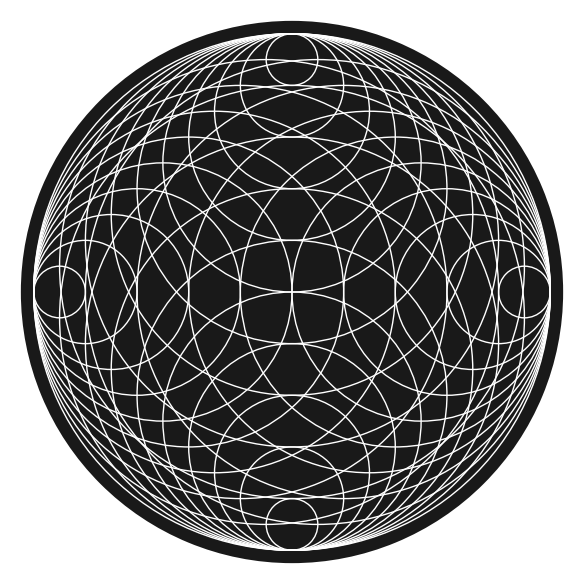
Interesting images - 2

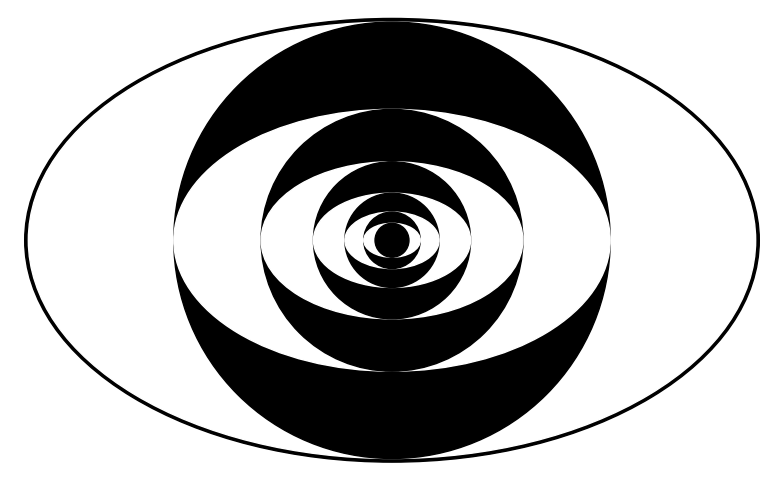
Let us command the computer to generate some more art!

Below is a modification from previous post.

1
2
3
4
5
6
7
plt=Graphics()
n = 5
plt += ellipse((0,0),5.05,3.05,fill=1,color='black')
for i in range(n+1):
    plt += ellipse((0,0),(3/5)^i*5,(3/5)^i*3,fill=1,color='white')
    plt += circle((0,0),(3/5)^i*3,color='black',fill=1)
plt.show(frame=0,axes=0)
../../images/eyes2.png

Fractal eyes

1
2
3
4
5
6
7
8
9
plt=Graphics()
n = 10
for i in range(1,n+1):
    plt += circle((0,1-i/n),1-i/n,color='white')
    plt += circle((i/n,1),1-i/n,color='white')
    plt += circle((-i/n,1),1-i/n,color='white')
    plt += circle((0,2-i/n),i/n,color='white')
plt += disk((0,1),1.05,(0,2*pi),color='black',alpha=0.9)
plt.show(frame=0,axes=0)
../../images/circles3.png

Circles!

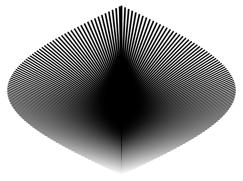
1
2
3
4
5
plt=Graphics()
n = 200
for i in range(1,n+1):
    plt += line2d([(0,i/n),((-1)^i*sin(pi/n*i),2*i/n)],color='black',thickness=(i/n)*n/50)
plt.show(frame=0,axes=0)
../../images/hood.png

What?

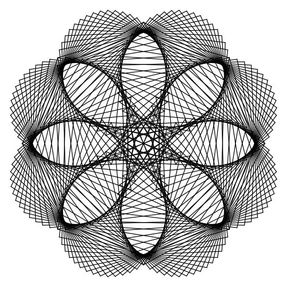
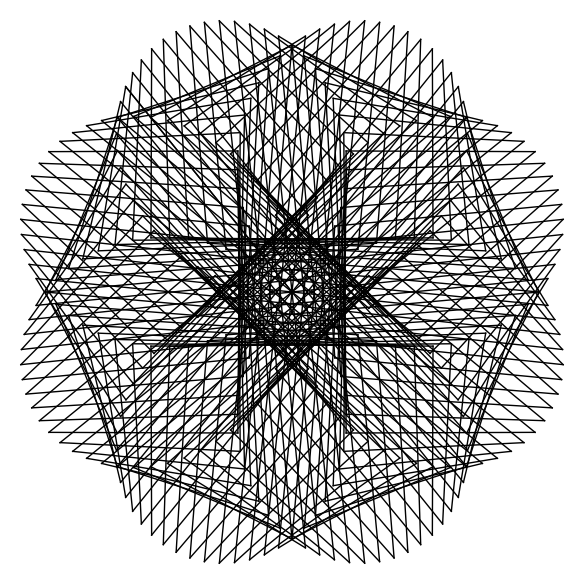
Some more, parametric plot using lines. Smooth edges are okay, few rough edges are a pain, many rough edges are soothing!

1
2
3
4
5
6
7
8
def draw(a,b,d):
    d=d*pi/180
    plt=Graphics()
    nn = 360
    for i in range(nn+1):
        plt += line2d([(sin(a*i*d)*sin(b*i*d),cos(a*(i)*d)*sin(b*(i)*d)),(sin(a*(i+1)*d)*sin(b*(i+1)*d),cos(a*(i+1)*d)*sin(b*(i+1)*d))],color='black')
    plt.show(frame=0,axes=0,aspect_ratio=1)
draw(3,4,11)
../../images/d37.png

\(d = 37\)

../../images/d107.png

\(d = 107\)

Change d to any other prime, also try changing a and b, there are many possibilities!

Interesting images using recurrences/iterations

Think of a simple figure. Now, think how it may look like if you repeat the same figure by placing it close to the original figure but smaller in size (e.g. by halving in size), and keep repeating.

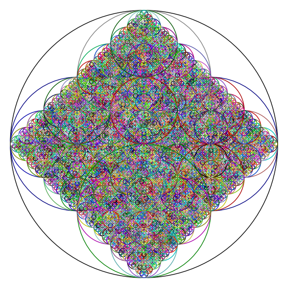
Here are some snippets of code in Sage to use the idea using circles, experiment with it by changing the parameters/shape.

var('y')
plt=Graphics()
a=22
b=22
def doit(a,b,ra,cnt):
    global plt
    plt += circle((a,b),ra,color=(randint(0,cnt)/(1+cnt),randint(0,cnt)/(1+cnt),randint(0,cnt)/(1+cnt)))
    if cnt >5:
        return
    doit(a+ra/2,a,ra/2,cnt+1)
    doit(a-ra/2,a,ra/2,cnt+1)
    doit(a,a-ra/2,ra/2,cnt+1)
    doit(a,a+ra/2,ra/2,cnt+1)
doit(0,0,22,0)
plt.show(frame=False,axes=0)
../../images/circles1.png

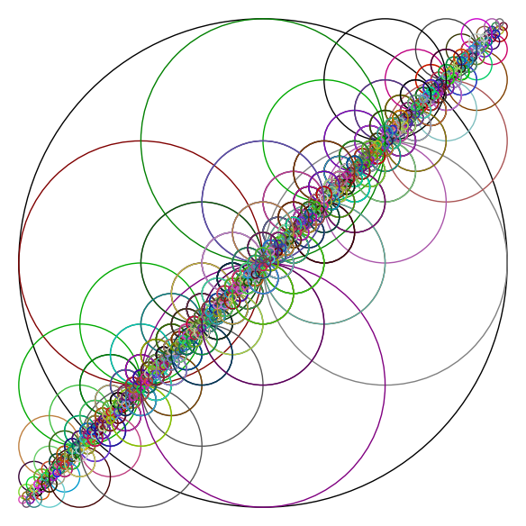
A saturn-like fractal

plt=Graphics()
a=22
b=22
def doit(a,b,ra,cnt):
    global plt
    plt += circle((a,b),ra,color=(randint(0,cnt)/(1+cnt),randint(0,cnt)/(1+cnt),randint(0,cnt)/(1+cnt)))
    if cnt > 5:
        return
    doit(a+ra/2,b,ra/2,cnt+1)
    doit(a-ra/2,b,ra/2,cnt+1)
    doit(a,b-ra/2,ra/2,cnt+1)
    doit(a,b+ra/2,ra/2,cnt+1)
doit(0,0,22,0)
plt.show(frame=False,axes=0)
../../images/circles2.png

Another fractal using circles

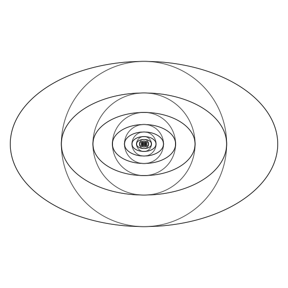
plt=Graphics()
a=16*golden_ratio
b=16
k=a/b
for i in range(11):
    plt += implicit_plot(x^2/a^2+y^2/b^2-1, (-a, a), (-a, a),color=(0,0,0))
    plt += implicit_plot(x^2/b^2+y^2/b^2-1, (-a, a), (-a, a),color=(.2,.2,.2))
    a = a/k
    b = b/k
plt.show(frame=False,axes=0)
../../images/eyes1.png

A fractal eye

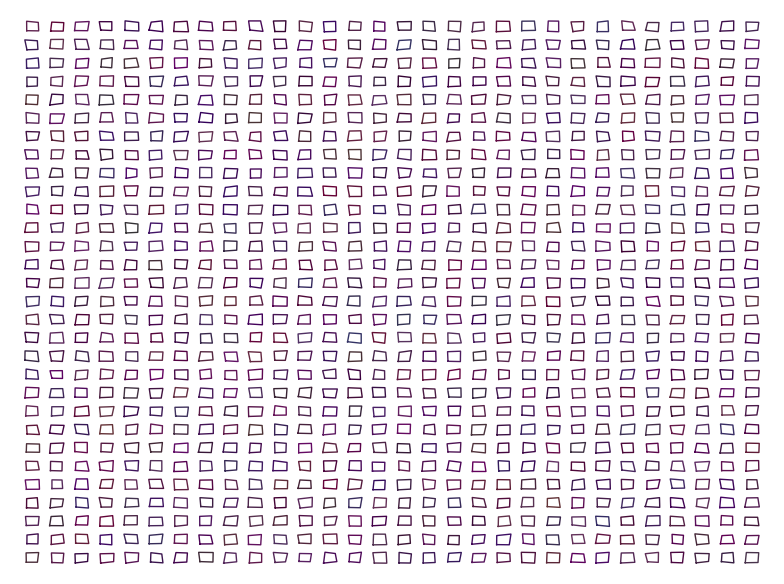
The below two are from Knuth's TAOCP vol 2 -- a little bit of randomness is good!

1
2
3
4
5
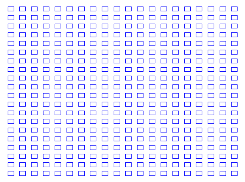
plt=Graphics()
for a in range(-20,20,2):
    for b in range(-20,20,2):
        plt += line([(a,b),(a+1,b),(a+1,b+1),(a,b+1),(a,b)])
plt.show(frame=0,axes=0)
../../images/tiles1.png

Regular tiles

1
2
3
4
5
6
7
8
plt=Graphics()
def ran(): return random()*0.2-0.1
for a in range(-20,40,2):
    for b in range(-20,40,2):
        x1=a+ran()
        y1=b+ran()
        plt += line([(x1,y1),(a+1+ran(),b+ran()),(a+1+ran(),b+1+ran()),(a+ran(),b+1+ran()),(x1,y1)],color=(ran()+0.3,ran()+0.1,ran()+0.3))
plt.show(frame=0,axes=0)
../../images/tiles2.png

Slightly randomized tiles